Subtraction Algorithm tutorial
This tutorial shows how to estimate the Galactic foregound of Galactic binaries
import os
import torch
import numpy as np
import matplotlib.pyplot as plt
plt.rcParams['font.size'] = 14
plt.rcParams['text.usetex'] = True
plt.rcParams['font.family'] = 'serif'

from corner import corner
from fast_lisa_subtraction import GalacticBinaryPopulation, SourceCatalog, SubtractionAlgorithm

# Specify the device to use for computations
device = 'cuda' if torch.cuda.is_available() else 'cpu'
Simulate a DWD Population
We first use the GalacticBinaryPopulation class to draw samples of a DWD Population.
This class uses the the parametrization explained in De Santi F. et al (2026) and is by default initialized to a fit to the catalog of Lamberts A. et al. (2019) which we will use for this example.
# Instantiate the GalacticBinaryPopulation class
GB_population = GalacticBinaryPopulation(device=device)

# Generate samples from the population
N = int(7e6)
GB_population_samples = GB_population.sample(N)

# Convert to a dataframe and inspect the columns
GB_population_df = GB_population_samples.dataframe()
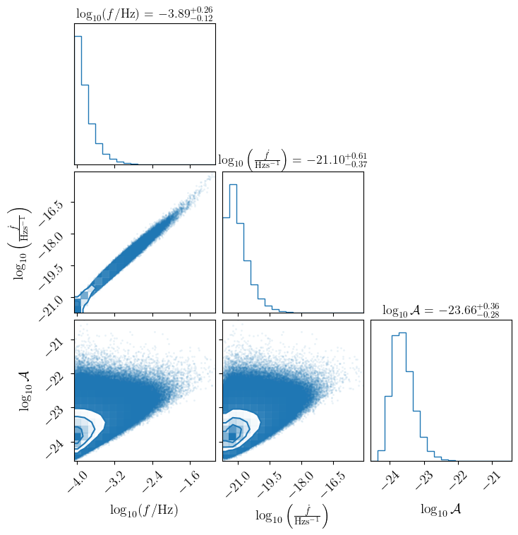
We then can plot the distribution in $(f, \dot{f}, \mathcal{A})$
samples_numpy = GB_population_samples.numpy()
plot_samples = np.log10(samples_numpy[:, [0, 1, 2]])

fig = corner(plot_samples,
             labels=[r'$\log_{10}(f/{\rm Hz})$', r'$\log_{10}\left(\frac{\dot{f}}{{\rm Hzs^{-1}}}\right)$', r'$\log_{10}\mathcal{A}$'],
             show_titles=True, color='C0', title_kwargs={'fontsize': 13})
[WARNING] - Too few points to create valid contours
Sources generation
We now generate the sources from the catalog above and inject into a LISA datastream.
We use SourceCatalog to generate and save the catalog.
We need to specify:
Nmax_binaries: Number of sources to generate. IfNone, the full catalog is generated.Nbatch: Number of sources processed per batch. This is useful to control memory usage, especially when running on GPU.Tobs: Observation time (in years).AET: IfTrue, the output is provided in the AET TDI basis.vOtherwise, the output may be in the XYZ basis.save: IfTrue, the generated catalog and/or time series are saved to disk.oversample: Oversampling factor used when generating the time series.tdi2: IfTrue, second-generation TDI (TDI 2.0) is used.outdir: Output directory where generated files will be stored.
This return as an output a dictionary with all the metadata and the TDI channels
catalog = SourceCatalog(catalog_df=GB_population_df, use_gpu=True if device=='cuda' else False)

AET = catalog.generate_catalogue(
    Nmax_binaries = None,
    Nbatch        = 10000,
    Tobs          = 4,
    AET           = True,
    save          = True,
    oversample    = 1,
    tdi2          = True,
    outdir        = os.getcwd(),
)

catalog_path = os.path.join(os.getcwd(), f'GB_catalogue_{N}_binaries.h5')
tdi_data_path = os.path.join(os.getcwd(), f'tdi_cat_GB_catalogue_{N}_binaries.h5')
[INFO] - Cupy is available: using the GPU
Generating waveforms: 100%|██████████| 700/700 [00:06<00:00, 102.46it/s]
[INFO] - Saving the catalogue with 7000000 binaries
[INFO] - TDI catalogue saved in /home/fdesanti/work/LISA/fast-lisa-subtraction/examples/tdi_cat_GB_catalogue_7000000_binaries.h5
[INFO] - Catalogue saved in /home/fdesanti/work/LISA/fast-lisa-subtraction/examples/GB_catalogue_7000000_binaries.h5
AET
{'A': array([ 6.56596047e-15-1.56411744e-14j, -1.51980682e-14-5.03222289e-15j,
        -2.26717721e-15-1.23868115e-14j, ...,
         0.00000000e+00+0.00000000e+00j,  0.00000000e+00+0.00000000e+00j,
         0.00000000e+00+0.00000000e+00j], shape=(4207754,)),
 'E': array([ 1.00297762e-14+1.32854742e-14j,  1.20677020e-14+1.85768499e-14j,
        -4.13275250e-15+5.53553918e-15j, ...,
         0.00000000e+00+0.00000000e+00j,  0.00000000e+00+0.00000000e+00j,
         0.00000000e+00+0.00000000e+00j], shape=(4207754,)),
 'T': array([ 1.04152541e-15-2.61888947e-14j, -1.00204175e-14-1.21080498e-14j,
         2.76406318e-14+9.74976982e-15j, ...,
         0.00000000e+00+0.00000000e+00j,  0.00000000e+00+0.00000000e+00j,
         0.00000000e+00+0.00000000e+00j], shape=(4207754,)),
 'f': array([0.00000000e+00, 7.92188395e-09, 1.58437679e-08, ...,
        3.33333151e-02, 3.33333230e-02, 3.33333309e-02], shape=(4207754,)),
 'df': 7.921883946719446e-09,
 'dt': 15,
 'Tobs': 126232599.05418241,
 'tdi2': True,
 'duty_cycle': 1,
 'oversample': 1,
 'snr': array([0.00315701, 0.0003168 , 0.0004559 , ..., 0.00751764, 0.00173092,
        0.00579411], shape=(7000000,))}
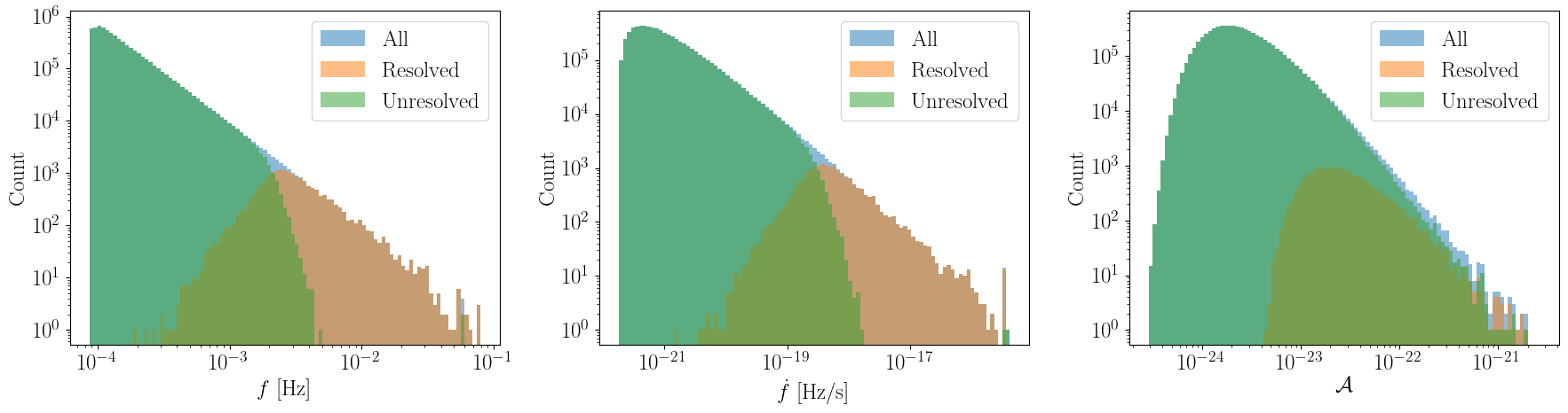
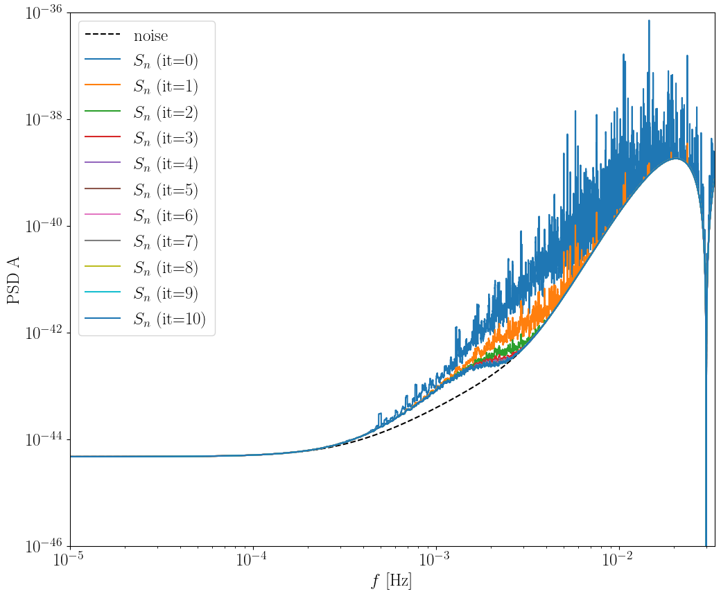
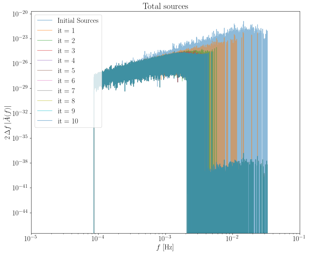
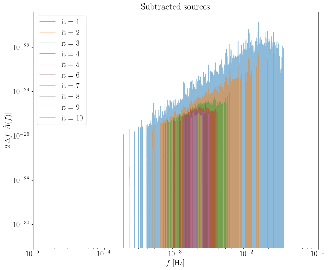
Running the Subtraction
We now run the subtraction algorithm. It returns:
out: output object containing the resolved sources and related products (e.g. waveforms / indices / parameters, depending on implementation)PSD: the estimated foreground (and/or residual) Power Spectral Densitycat_figs: diagnostic figures produced during the run (ifdoplot=True)
We need to specify:
maxiter: Maximum number of subtraction iterations.snr_threshold: Signal-to-noise ratio threshold used to classify sources as resolved.kappa: sources with initialkappa*snr_thresholdsnr are left out from the subtraction. Assumeskappa<= 1doplot: IfTrue, generates diagnostic plots during/after the run and returns them incat_figs.batch_size: Number of sources processed per internal batch during the subtraction step.methoduse: Method usedto estimate the PSD (either “mean” or “median”)extra_smooth: Additional smoothing strategy applied to the PSD estimate. For example “convolution” applies a kernel-based smoothing to reduce small-scale fluctuations.Nsegments: Number of segments used to estimate the PSDtol: Convergence tolerance. The algorithm stops early if the change in the PSD drops below this value.verbose: IfTrue, prints progress information and iteration diagnostics.
# Initialize the subtraction algorithm
subtract = SubtractionAlgorithm(catalog_path  = catalog_path,
                                tdi_data_path = tdi_data_path ,
                                use_gpu       = True if device == 'cuda' else False)

# Run the subtraction
out, PSD, cat_figs = subtract.run(
      maxiter       = 10,
      snr_threshold = 7,
      kappa         = 0.15,
      doplot        = True,
      batch_size    = 1000,
      methoduse     = 'mean',
      extra_smooth  = "convolution",
      Nsegments = 2000,
      tol       = 1e-3,
      verbose   = True
)

display(cat_figs)
[INFO] - Cupy is available: using the GPU
[INFO] - Reading catalogue data from /home/fdesanti/work/LISA/fast-lisa-subtraction/examples/GB_catalogue_7000000_binaries.h5
[INFO] - Catalogue contains 7000000 sources
/home/fdesanti/miniconda3/envs/lisa/lib/python3.10/site-packages/cupyx/jit/_interface.py:173: FutureWarning: cupyx.jit.rawkernel is experimental. The interface can change in the future.
  cupy._util.experimental('cupyx.jit.rawkernel')
[INFO] - Starting the local subtraction algorithm
[INFO] - Minimum SNR = 0.00005, maximum SNR = 3401.39
[INFO] - Selecting sources with SNR > 1.05
[INFO] - Selecting 88059/7000000 sources for subtraction
[INFO] - Initial PSD computed
[INFO] - Making initial plot
  0%|          | 0/10 [00:00<?, ?it/s][INFO] - Starting iteration 1
100%|==========================================| 88/88 [00:00<00:00, 241.60it/s]
[INFO] - Subtracted sources: 7509
[INFO] - 7509 source subtracted at iter 1.
[INFO] - New PSD computed
[INFO] - Making plot for iteration 1
 10%|█         | 1/10 [00:02<00:21,  2.37s/it][INFO] - Starting iteration 2
100%|==========================================| 80/80 [00:00<00:00, 258.62it/s]
[INFO] - Subtracted sources: 6399
[INFO] - 6399 source subtracted at iter 2.
[INFO] - New PSD computed
[INFO] - Making plot for iteration 2
 20%|██        | 2/10 [00:05<00:22,  2.78s/it][INFO] - Starting iteration 3
100%|==========================================| 74/74 [00:00<00:00, 256.14it/s]
[INFO] - Subtracted sources: 2762
[INFO] - 2762 source subtracted at iter 3.
[INFO] - New PSD computed
[INFO] - Making plot for iteration 3
 30%|███       | 3/10 [00:09<00:22,  3.21s/it][INFO] - Starting iteration 4
100%|==========================================| 71/71 [00:00<00:00, 258.44it/s]
[INFO] - Subtracted sources: 951
[INFO] - 951 source subtracted at iter 4.
[INFO] - New PSD computed
[INFO] - Making plot for iteration 4
 40%|████      | 4/10 [00:13<00:22,  3.70s/it][INFO] - Starting iteration 5
100%|==========================================| 70/70 [00:00<00:00, 257.30it/s]
[INFO] - Subtracted sources: 304
[INFO] - 304 source subtracted at iter 5.
[INFO] - New PSD computed
[INFO] - Making plot for iteration 5
 50%|█████     | 5/10 [00:18<00:21,  4.24s/it][INFO] - Starting iteration 6
100%|==========================================| 70/70 [00:00<00:00, 260.78it/s]
[INFO] - Subtracted sources: 116
[INFO] - 116 source subtracted at iter 6.
[INFO] - New PSD computed
[INFO] - Making plot for iteration 6
 60%|██████    | 6/10 [00:24<00:19,  4.80s/it][INFO] - Starting iteration 7
100%|==========================================| 70/70 [00:00<00:00, 270.60it/s]
[INFO] - Subtracted sources: 39
[INFO] - 39 source subtracted at iter 7.
[INFO] - New PSD computed
[INFO] - Making plot for iteration 7
 70%|███████   | 7/10 [00:31<00:16,  5.39s/it][INFO] - Starting iteration 8
100%|==========================================| 69/69 [00:00<00:00, 273.21it/s]
[INFO] - Subtracted sources: 13
[INFO] - 13 source subtracted at iter 8.
[INFO] - New PSD computed
[INFO] - Making plot for iteration 8
 80%|████████  | 8/10 [00:38<00:12,  6.04s/it][INFO] - Starting iteration 9
100%|==========================================| 69/69 [00:00<00:00, 277.31it/s]
[INFO] - Subtracted sources: 8
[INFO] - 8 source subtracted at iter 9.
[INFO] - New PSD computed
[INFO] - Making plot for iteration 9
 90%|█████████ | 9/10 [00:46<00:06,  6.73s/it][INFO] - Starting iteration 10
100%|==========================================| 69/69 [00:00<00:00, 278.86it/s]
[INFO] - Subtracted sources: 4
[INFO] - 4 source subtracted at iter 10.
[INFO] - New PSD computed
[INFO] - Making plot for iteration 10
100%|██████████| 10/10 [00:55<00:00,  5.59s/it]
[INFO] - Subtraction algorithm took  56.9 seconds and 10 iterations
[INFO] - Total subtracted sources: 18105
print(out.keys())
out
dict_keys(['A', 'E', 'T', 'Tobs', 'df', 'dt', 'duty_cycle', 'f', 'oversample', 'snr', 'tdi2', 'A_original', 'E_original', 'T_original', 'resolved_cat', 'unresolved_cat', 'num_sources', 'num_resolved', 'num_unresolved', 'runtime', 'iterations', 'Sconf'])
{'A': array([ 1.23750521e-17-1.21146037e-18j,  2.30985640e-18-1.13647080e-18j,
        -1.58123886e-17-8.88589963e-19j, ...,
         0.00000000e+00+0.00000000e+00j,  0.00000000e+00+0.00000000e+00j,
         0.00000000e+00+0.00000000e+00j], shape=(4207754,)),
 'E': array([3.02035570e-18+3.23866884e-18j, 5.63116374e-18+2.33177858e-18j,
        4.34558100e-18+4.44667121e-19j, ...,
        0.00000000e+00+0.00000000e+00j, 0.00000000e+00+0.00000000e+00j,
        0.00000000e+00+0.00000000e+00j], shape=(4207754,)),
 'T': array([1.33224648e-17-9.47084378e-18j, 1.80744821e-17+2.67857440e-17j,
        7.44929416e-18+1.43022934e-17j, ...,
        0.00000000e+00+0.00000000e+00j, 0.00000000e+00+0.00000000e+00j,
        0.00000000e+00+0.00000000e+00j], shape=(4207754,)),
 'Tobs': array(1.26232599e+08),
 'df': array(7.92188395e-09),
 'dt': array(15),
 'duty_cycle': array(1),
 'f': array([0.00000000e+00, 7.92188395e-09, 1.58437679e-08, ...,
        3.33333151e-02, 3.33333230e-02, 3.33333309e-02], shape=(4207754,)),
 'oversample': array(1),
 'snr': array([0.00257776, 0.01005576, 0.00313661, ..., 0.00032715, 0.00663081,
        0.00218669], shape=(7000000,)),
 'tdi2': array(True),
 'A_original': array([-1.58778639e-14-1.84461216e-15j, -1.17925776e-14-4.98779250e-15j,
         6.47146614e-15+8.37014176e-16j, ...,
         0.00000000e+00+0.00000000e+00j,  0.00000000e+00+0.00000000e+00j,
         0.00000000e+00+0.00000000e+00j], shape=(4207754,)),
 'E_original': array([4.20337088e-15+3.27932766e-15j, 9.41571528e-15+7.01742681e-15j,
        9.03612106e-15+2.18168864e-15j, ...,
        0.00000000e+00+0.00000000e+00j, 0.00000000e+00+0.00000000e+00j,
        0.00000000e+00+0.00000000e+00j], shape=(4207754,)),
 'T_original': array([-8.88697899e-16+7.95363426e-16j,  7.06311032e-15+1.97869977e-14j,
         1.35028886e-14+1.39751369e-14j, ...,
         0.00000000e+00+0.00000000e+00j,  0.00000000e+00+0.00000000e+00j,
         0.00000000e+00+0.00000000e+00j], shape=(4207754,)),
 'resolved_cat':           Amplitude  EclipticLatitude  EclipticLongitude  Frequency  \
 0      7.461294e-23         -0.684062          -3.279134   0.006245
 1      2.678701e-23          0.001691          -3.508877   0.002391
 2      8.617990e-23          0.003610          -3.014246   0.001178
 3      3.814219e-23         -0.003226          -3.219182   0.013113
 4      5.188652e-23          0.096143          -3.115334   0.003120
 ...             ...               ...                ...        ...
 18100  1.916361e-23         -0.725985          -3.048061   0.002124
 18101  8.921188e-24         -0.023322          -3.179191   0.002337
 18102  2.448078e-23          0.016256          -2.855514   0.001934
 18103  1.889485e-23          0.176347          -3.335850   0.001924
 18104  1.451972e-23         -0.122610          -3.069855   0.001937

        FrequencyDerivative  Inclination  InitialPhase  Polarization
 0             2.674486e-18     0.963475      0.866809      3.106331
 1             2.896236e-19     2.333052      6.269701      5.975049
 2             9.796302e-20     2.825798      3.798167      3.311297
 3             1.212599e-17     2.497385      5.209013      5.619650
 4             5.398476e-19     2.430412      2.046115      5.964725
 ...                    ...          ...           ...           ...
 18100         3.603896e-19     1.816379      5.024586      2.360944
 18101         4.934780e-19     2.256582      2.880993      3.383741
 18102         2.075758e-19     1.747774      0.473650      3.743894
 18103         1.285527e-19     2.008865      4.982120      2.353525
 18104         1.960376e-19     0.908985      3.370217      4.134227

 [18105 rows x 8 columns],
 'unresolved_cat':             Amplitude  EclipticLatitude  EclipticLongitude  Frequency  \
 0        2.184889e-24          0.052374          -3.986333   0.000120
 1        2.456927e-24         -0.211355          -3.172136   0.000262
 2        4.793424e-24         -0.013430          -3.155939   0.000108
 3        7.004272e-25         -0.065210          -3.090360   0.000115
 4        6.643289e-24         -0.101062          -3.111741   0.000098
 ...               ...               ...                ...        ...
 6981890  1.727319e-23         -0.001962          -3.375396   0.000874
 6981891  6.022181e-23          0.452347          -3.129454   0.000592
 6981892  1.409613e-23         -0.106831          -2.657236   0.000679
 6981893  1.653164e-23          0.065999          -2.952805   0.001094
 6981894  1.323182e-23          0.293619          -3.382494   0.001322

          FrequencyDerivative  Inclination  InitialPhase  Polarization
 0               7.488707e-22     2.862180      4.312956      5.612725
 1               4.299681e-21     1.403915      3.339834      0.232345
 2               4.834366e-22     0.782177      3.492598      5.361196
 3               5.377511e-22     2.019329      1.844765      5.675665
 4               3.467041e-22     0.877479      0.611017      2.957046
 ...                      ...          ...           ...           ...
 6981890         4.556329e-20     0.682707      0.039144      5.701773
 6981891         2.159866e-20     1.208989      1.504324      3.662067
 6981892         5.738881e-20     0.508316      3.795960      2.757061
 6981893         5.941227e-20     1.532906      2.418825      4.659492
 6981894         1.054291e-19     0.982424      3.750560      4.067661

 [6981895 rows x 8 columns],
 'num_sources': 7000000,
 'num_resolved': 18105,
 'num_unresolved': 6981895,
 'runtime': 56.88103461265564,
 'iterations': 10,
 'Sconf': {'A': array([           nan, 1.19543763e-43, 1.34663315e-43, ...,
         7.45706069e-40, 7.45709522e-40, 7.45712975e-40], shape=(4207754,)),
  'E': array([           nan, 6.48186813e-44, 7.27336007e-44, ...,
         7.45706069e-40, 7.45709522e-40, 7.45712975e-40], shape=(4207754,)),
  'T': array([           nan, 7.34294320e-43, 8.30965184e-43, ...,
         9.62834647e-40, 9.62839661e-40, 9.62844676e-40], shape=(4207754,))}}