Simulating catalogs

This tutorial shows how to generate mock catalogs of Galactic binaries

import os
import torch
import numpy as np
import matplotlib.pyplot as plt
plt.rcParams['font.size'] = 14
plt.rcParams['text.usetex'] = True
plt.rcParams['font.family'] = 'serif'

from corner import corner
from fast_lisa_subtraction.utils import latexify

# Specify the device to use for computations
device = 'cuda' if torch.cuda.is_available() else 'cpu'

Simulate a DWD Population

We will make use of the GalacticBinaryPopulation class to draw samples of a DWD Population.

This class uses enables the sampling of the parameters describing a catalog of GBs

In particular:

• Frequency

• FrequencyDerivative

• Amplitude

• InitialPhase

• Inclination

• Polarization

• EclipticLatitude

• EclipticLongitude

the the parametrization explained in De Santi F. et al (2026) and is by default initialized to reproduce the best fit to the catalog of Lamberts A. et al. (2019)

Priors

FastLisaSubtraction supports multiple analytical priors, like Uniform, Gaussian, Gamma, LogNormal as described in De Santi F. et al (2026)

import fast_lisa_subtraction.priors as priors

print(priors.__all__)

['Uniform', 'LogNormal', 'Gamma', 'PowerLaw', 'BrokenPowerLaw', 'UniformCosine', 'UniformSine', 'Gaussian', 'Cauchy', 'GalacticBinaryPopulation']

In order to generate a mock catalog we need to instanciate the GalacticBinaryPopulation class.

We first need to define a dictionary with the prior for each set of parameters, as an example:

from fast_lisa_subtraction.priors import *

prior_dict = dict(
                Frequency           = PowerLaw(alpha=-2, minimum=1e-4, maximum=1e-1, name='Frequency', device=device),
                FrequencyDerivative = Gamma(alpha=2, beta=3, offset=-20.0, name='FrequencyDerivative', device=device),
                Amplitude           = LogNormal(mu=-21.5, sigma=0.2, minimum=-24.5, maximum=-20.5, name='Amplitude', device=device),
                InitialPhase        = Uniform(0, 2*np.pi, name='InitialPhase', device=device),
                Inclination         = UniformCosine(0, np.pi, name='Inclination', device=device),
                Polarization        = Uniform(0, 2*np.pi, name='Polarization', device=device),
                EclipticLatitude    = UniformSine(-np.pi/2, np.pi/2, name='EclipticLatitude', device=device),
                EclipticLongitude   = Uniform(0, 2*np.pi, name='EclipticLongitude', device=device)
            )

Then we use the class to sample the marginal and introduce a copula correlation in $f$-$\dot{f}$ as described in De Santi F. et al (2026)

Other available copulas are the Clayton, Frank and Student-T, refer to the documentation page for details

# Instantiate the GalacticBinaryPopulation class
GB_population = GalacticBinaryPopulation(priors=prior_dict, device=device)

# Generate samples from the population
N = int(1e6)
GB_population_samples = GB_population.sample(N, copula=True, kind='gaussian', rho=0.8)

# Convert to a dataframe and inspect the columns
GB_population_df = GB_population_samples.dataframe()

GB_population_df.head()

	Frequency	FrequencyDerivative	Amplitude	InitialPhase	Inclination	Polarization	EclipticLatitude	EclipticLongitude
0	0.000102	9.838469e-21	1.047984e-23	5.581181	2.062936	2.949006	-0.684814	6.278080
1	0.001257	2.889604e-20	2.848996e-22	5.217888	2.465560	4.257358	-0.258646	4.241662
2	0.000104	5.488845e-21	4.679115e-24	3.888970	0.441004	5.520145	-0.408062	5.351471
3	0.000134	7.041943e-21	4.371890e-24	2.507201	1.304868	4.035791	-0.428621	1.592792
4	0.000255	8.474385e-21	2.026280e-23	1.373542	2.880041	2.436864	0.307664	2.670212

GB_population_samples.numpy().shape

(1000000, 8)

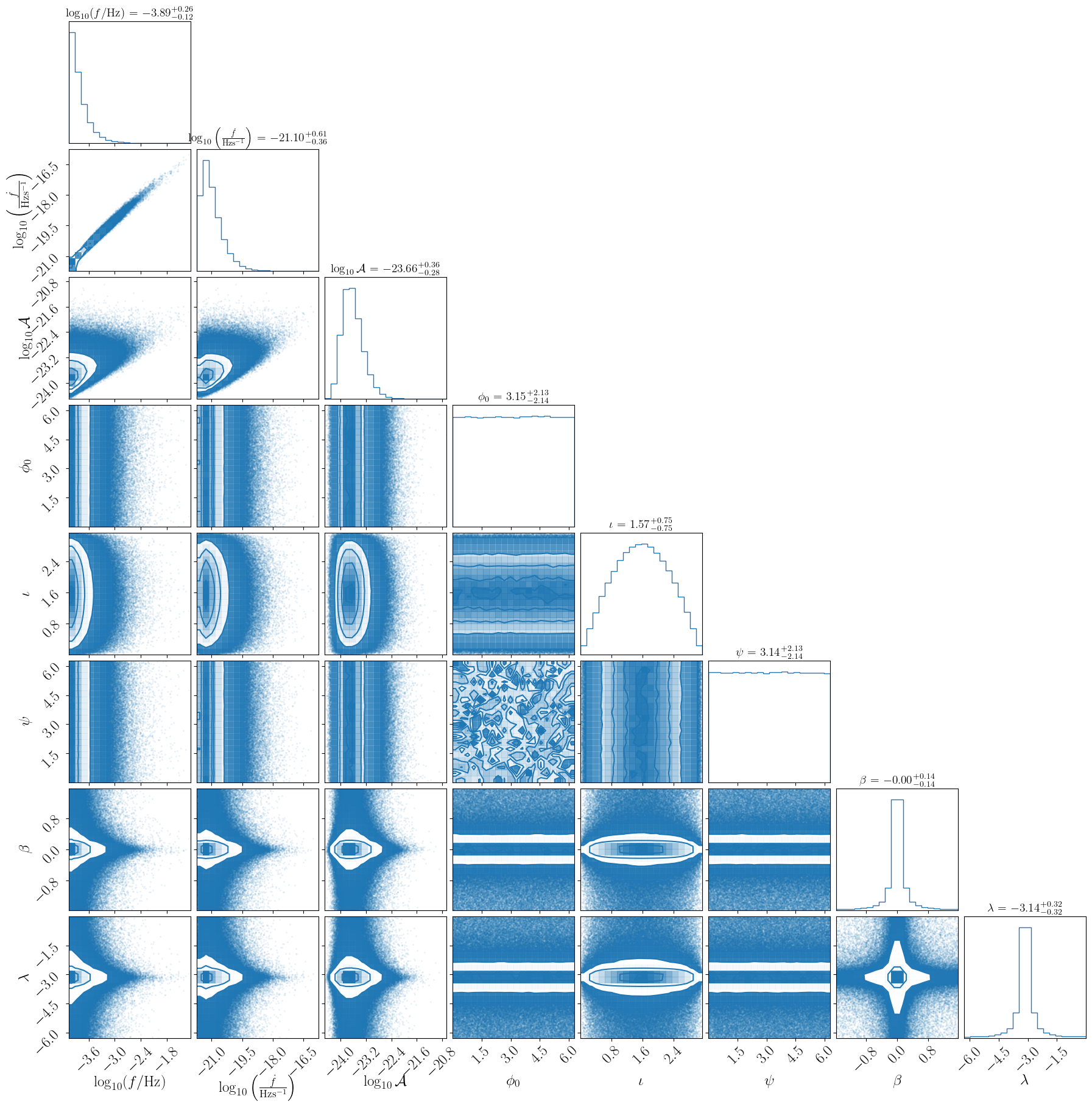
We then can plot the distributions

import copy
from fast_lisa_subtraction.utils import latexify

latex_dict = {
    'Frequency': r'$\log_{10}(f/{\rm Hz})$',
    'FrequencyDerivative': r'$\log_{10}\left(\frac{\dot{f}}{{\rm Hzs^{-1}}}\right)$',
    'Amplitude': r'$\log_{10}\mathcal{A}$',
    'InitialPhase': r'$\phi_0$',
    'Inclination': r'$\iota$',
    'Polarization': r'$\psi$',
    'EclipticLatitude': r'$\beta$',
    'EclipticLongitude': r'$\lambda$',
}

@latexify
def plot_catalogue(pop_samples, **corner_kwargs):
    pop_samples = copy.deepcopy(pop_samples)

    for key in ['Frequency', 'FrequencyDerivative', 'Amplitude']:
        pop_samples[key] = copy.deepcopy(torch.log10(pop_samples[key]))
    
    pop_samples_numpy = pop_samples.numpy()
    latex_labels = [latex_dict[key] for key in pop_samples.keys()]
    
    return corner(pop_samples_numpy, labels=latex_labels, **corner_kwargs)

fig = plot_catalogue(GB_population_samples, color='C0', plot_datapoints=True, show_titles=True, title_kwargs={'fontsize': 13})

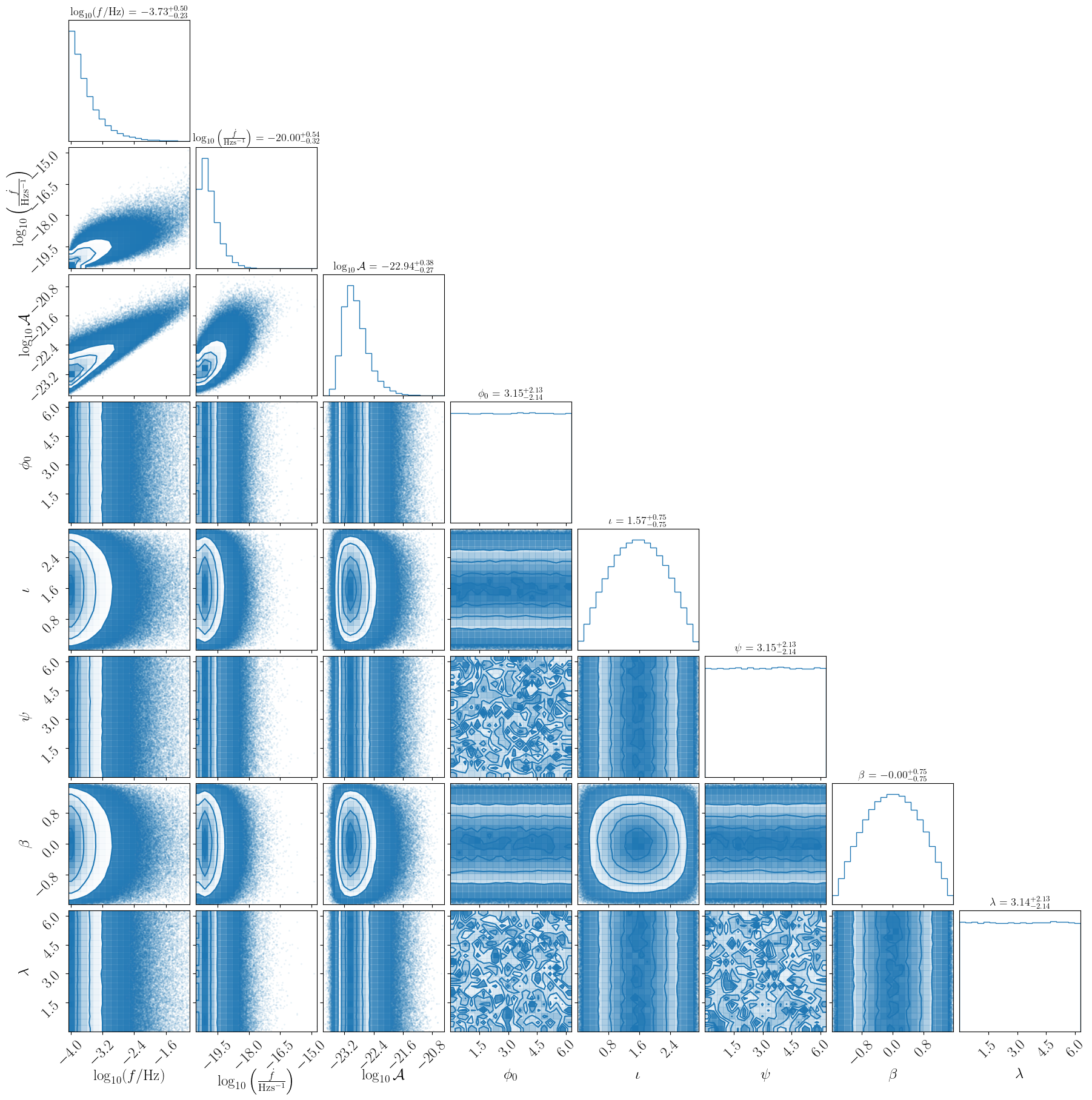
The class is by default initialized to reproduce a fit to the catalog of Lamberts A. et al. (2019).

# Instantiate the GalacticBinaryPopulation class
GB_population = GalacticBinaryPopulation(device=device)

# Generate samples from the population
GB_population_samples = GB_population.sample(N)

# Convert to a dataframe and inspect the columns
GB_population_df = GB_population_samples.dataframe()

fig = plot_catalogue(GB_population_samples, color='C0', plot_datapoints=True, show_titles=True, title_kwargs={'fontsize': 14})

[WARNING] - Too few points to create valid contours